Using Photoshop for Stream Table Image Analysis

Yet another wonderful thing about the color-coded plastic media is the ability to analyze stream features over time. The colors tend to organize themselves into patterns based on where the water is flowing that correspond to areas of erosion, transport, and deposition. My hope is that I can use these colors to define active/abandoned channels in each time lapse frame - stacking frames will show how those channel patterns over time. But how to simplify the images? One of the challenges lies in the fact that the yellow sediment contains some red hues - a simple saturation boost would make the yellows pop out too much. So I grabbed a picture of the stream table and tried out some Photoshop filters and adjustments to simplify the image. I've put them into an animated gif to show the differences.

I've noticed that the smallest red grains tend to show up in areas of scouring, while the white and yellow are often the first to move and the first to be deposited. Some of these adjustments really help pull out the yellow and red. Now it's time to get a time-lapse sequence and try some time series analysis.

Even more grain data

I finished the sieve analysis of the Emriver coded media. I pulled about a quart of material from each of the five buckets that were delivered (about 650 g per sample) for a total of 3.2 kg sieved material.

 I have also been analyzing the sieved fractions for specific gravity (SG). As mentioned before, I noticed the white material was yielding lower SG values than the other colors. Steve Gough suggested that I let the material soak a little longer. I had done that with a few samples, but I've started to let them soak overnight. The white material is still producing slightly lower values than the yellow, brown, or red. Here's a summary of the results so far (the two lowest SG values weren't soaked overnight):

Here's a set of bulk sediment measurements - I think the effect of not soaking them overnight is yielding a few slightly lower measurements, but the results suggest a bulk SG of about 1.53 - just a little shy of what the LRRD folks report (1.55).

Emriver color-coded sediment, un-mixing the media.

My soil mechanics students had their grain size analysis lab this week. It's fun - they get to analyze granular materials by playing with sand. Specifically, the plastic sand that comes standard with the Em2 stream table. Last year I ran the standard media through a stack of sieves. This year, I ran the color-coded plastic media through the sieves.

These gradation curves are a quick way of describing and comparing different sediments. The standard media (blue curve) is different by having a little bit less material between 2 and 1mm in size (but more material larger than 2.4mm), and quite a bit more fine material around 0.5mm. The horizontal axis is in microns (1 mm = 1,000 microns) and it's on a log scale, because there's such a huge range in diameter.

Here's a frequency curve showing the relative proportions of various size fractions. The "Phi Value" is another way sedimentologists scale the wide range of particles (Phi Value = -log₂diameter in mm). So the Phi Value of a sand grain 1 mm in diameter is zero. Notice the big bump in the standard media between 1.5 and 2 phi. My own speculation is that as the material moves around, the big particles grind themselves down into particles around this size (0.3mm).

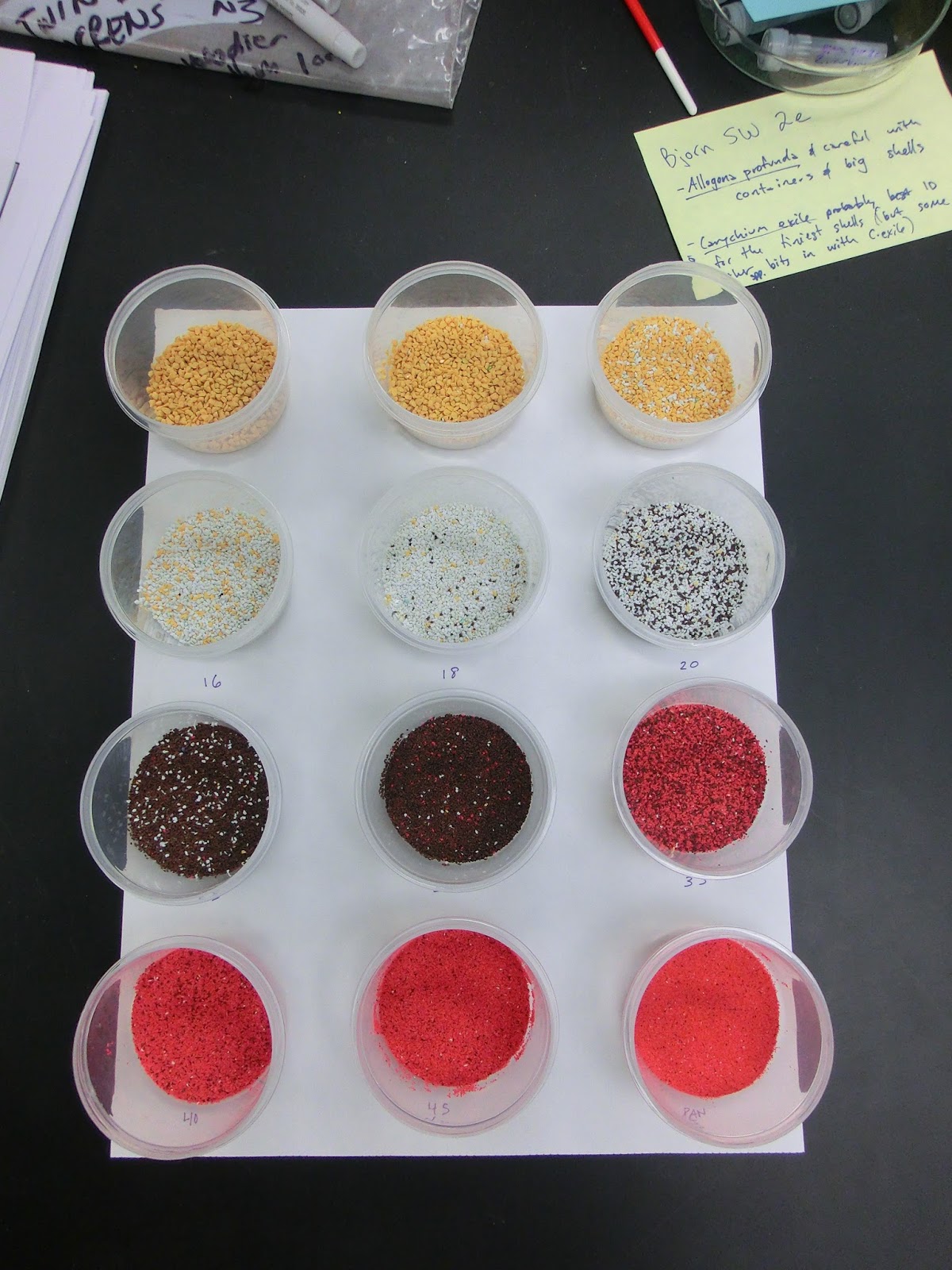
What you can't see, and what is the true brilliance behind the color-coded material, is how moving water separates the color-coded particles into various color patterns. You can also see the colors in the sieve separates, too.

So let's look at the distribution of grain sizes in the color coded media a little more closely:

 I like the distribution graph (given a little bit of visual "boost" by arbitrarily smoothing the line graph in Excel) because it hints at the formula for the Emriver sediment. There are four "bumps" that correspond to the sizes of the four different colors (Yellow = 1.4mm, White = 1mm, Brown = 0.7mm, Red = 0.4mm).

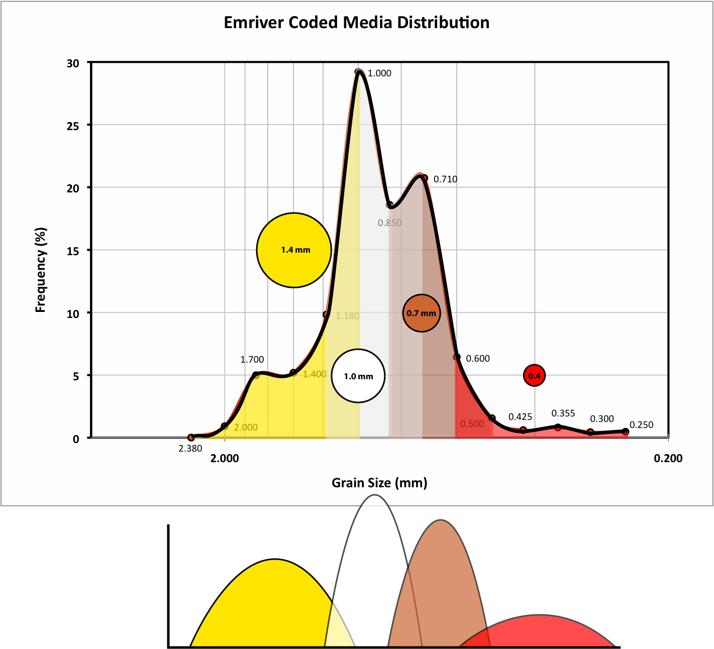
Here's an overlay of the color fractions - the curves below represent approximate distributions of each individual fraction.

Here's a picture from Steve, the big guy at LRRD's blog (Riparian Rap), showing the Em4 being filled with unmixed coded media. Given that some of the smallest yellow particles are smaller than the largest white particles, un-mixing the coded media into perfect color fractions isn't possible by mechanical means alone.

My plan now: use the grain size distributions to create "color facies" for the plastic media - providing a way to do grain size analysis with time lapse photographs.

Update: talking with Steve over email, I realized that the color fraction "curves" as drawn above may imply more quantitative "knowledge" than I really have about the distribution of each color. Here's a histogram, with the color fractions approximated by visually estimating the proportion of different colors visible in each container (vertical scale is in grams):

Slow-Mo Sedimentation: When Stokes' Law Doesn't Apply

Thanks to the ever helpful folks at LRRD, the colored sediment for my lab's Em2 arrived last week. I shot some high speed video of a scoop falling through water. Based on the results, I tried again with the help of my colleague Todd Zimmerman. We tried a few different colored gels on the translucent backdrop, but the first one that I used, a nice deep blue, works the best. I think it's because of the red-orange hues in all of the sediment particle sizes contrast well with the blue.

Colored sediment: when Stokes Law does not apply from Matt Kuchta on Vimeo.

Contrast this video with the footage we captured a few years ago of ball bearings falling through corn syrup:
What a Drag! Falling Through Syrup from Matt Kuchta on Vimeo.

The single ball bearing is a good example of how Stokes' Law works. I blogged about it before, too. But the first video shows many particles. These particles are banging into each other, the combined mass of the particles is also pushing the water around in turbulent eddies. Stokes' Law does not apply because the settling of each particle is hindered by interactions with other particles and the surrounding fluid. In these cases, we're often without a simple, elegant equation to describe what's happening. Instead, we have to rely on empirical observations. Such as the bedforms left behind in the sediments after the particles are deposited. In the end, however, many of the smallest particles are left behind to drape over the entire pile of material. So even in these chaotic, turbulent systems, Stokes' observations can still help inform us of these processes.

Emriver Color-Coded sediment in action

A little test run with the new color-coded sediment that arrived last week. It's so pretty!

I seem to recall some fluvial stratigraphy diagrams tossing around facies patterns that look strikingly similar.

I'm rather excited about 3D facies mapping possibilities here. Too bad I have so many other irons in the fire. 

Sediment Transport Porn

I think I've found the right material to use in high-speed video of sediment transport.

A link for aggregate readers that may cut things off: https://vimeo.com/60882601

The color-coded media supplied by Little River Research and Design looks absolutely gorgeous. I got some the other day and I just had to grab a few scoops to shoot some video friday afternoon:

Color-Coded Sediment from Matt Kuchta on Vimeo.
Some new material arrived in the lab today. Just a quick clip of a scoop of the color-coded sediment settling onto the bottom of a glass of water.